It’s been almost a year since the events described in a previous post of mine occurred.1Actually, the person whom that post involved really did not like that blog post. I actually asked our close mutual friend to send it to her (since we were and are in a weird point of our relationship where we aren’t talking to each other, despite our mutual friends’ assurances that we both are—in fact—still friends. [It’s a long story and actually the inspiration of a new short story I’ve been working on during the whole Covid-quarantine thing, so be on the look out. But I digress.]) and she did not like it at all. She took the line where I said “what a colossal waste of time that was” as a reference to her. Like our whole friendship was a waste of time. In fact, I wrote the thing with the idea that it might improve our relationship, if anything. I imagine if she reads this article (and this footnote in particular) that it would rather harm our already struggling relationship. The good news is that nobody seems to read these at all, so the probability that happens is small. Now you may be wondering: Colin, why would you post this at all if you know it would make her upset? Well… I really don’t know. ¯\_(ツ)_/¯ I’ve spent that time working and a nice side effect of my job is that I got to learn a good amount of probability theory. And so, at the approximate one year anniversary mark, I’d like to amend how I described the uncertainty of the probability of winning a game of clock solitaire. To do a more precise job of modeling it, we really should have used a beta distribution. For an (unfinished as of now) introduction in using the beta distribution to model probabilities, I suggest you watch the always excellent 3Blue1Brown’s videos on it.
So if we recall, my friend played twenty or so games and one a quarter of them which is a convoluted way of saying five. When we let our alpha parameter be 5 and our beta parameter be 15, we get the following plot of our beta distribution:
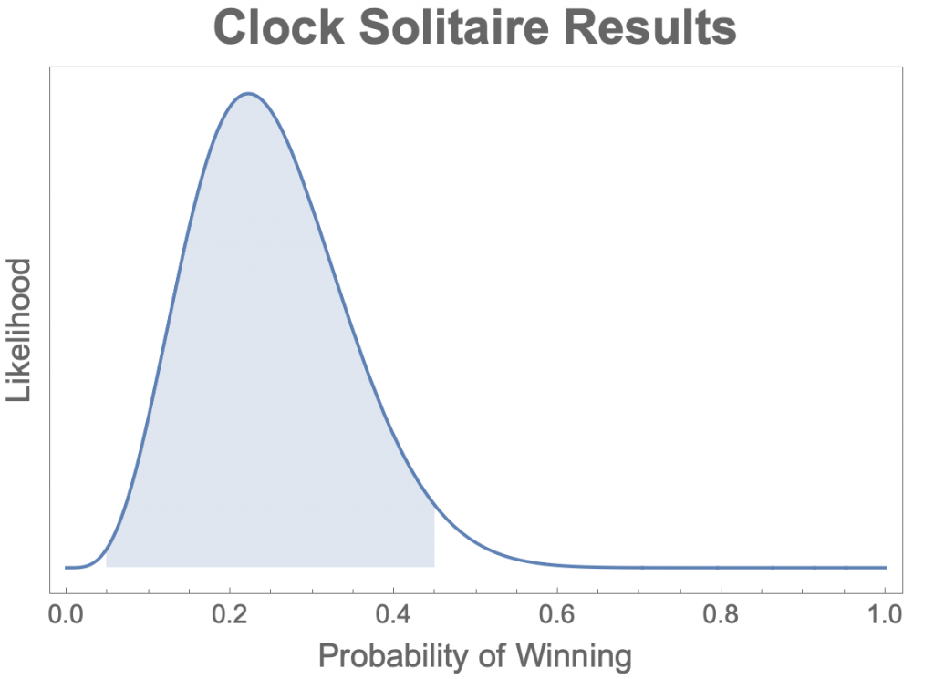
Now, since this is a probability distribution, that blue area needs to equal one. If we want to gather the interval of probabilities that will correspond to roughly 97% of the time, we need to find the interval of the probability ranges which corresponds to between an area of 0.97. Almost exactly 97% of the this distribution lies between a probability of 0.05 and 0.45. In other words, we expect the true probability of winning a random game of clock solitaire to be contained within 0.05 and 0.45 with a 97% confidence interval.
Now when we compare this to my trillion results of simulated data and make a plot, we get
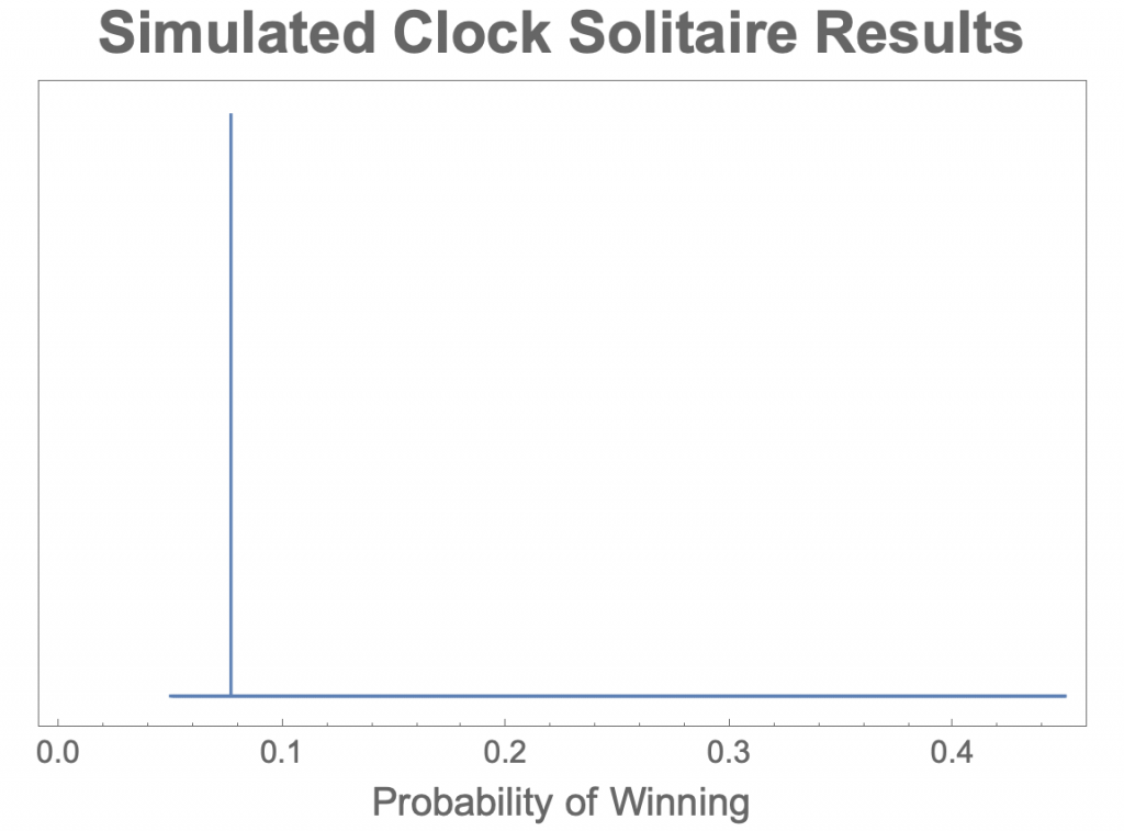
Hmmm…. I think we should zoom in a bit. (Note the change in the x-axis and forgive me for my lack of a y-axis label—it’s supposed to be “Likelihood”.)
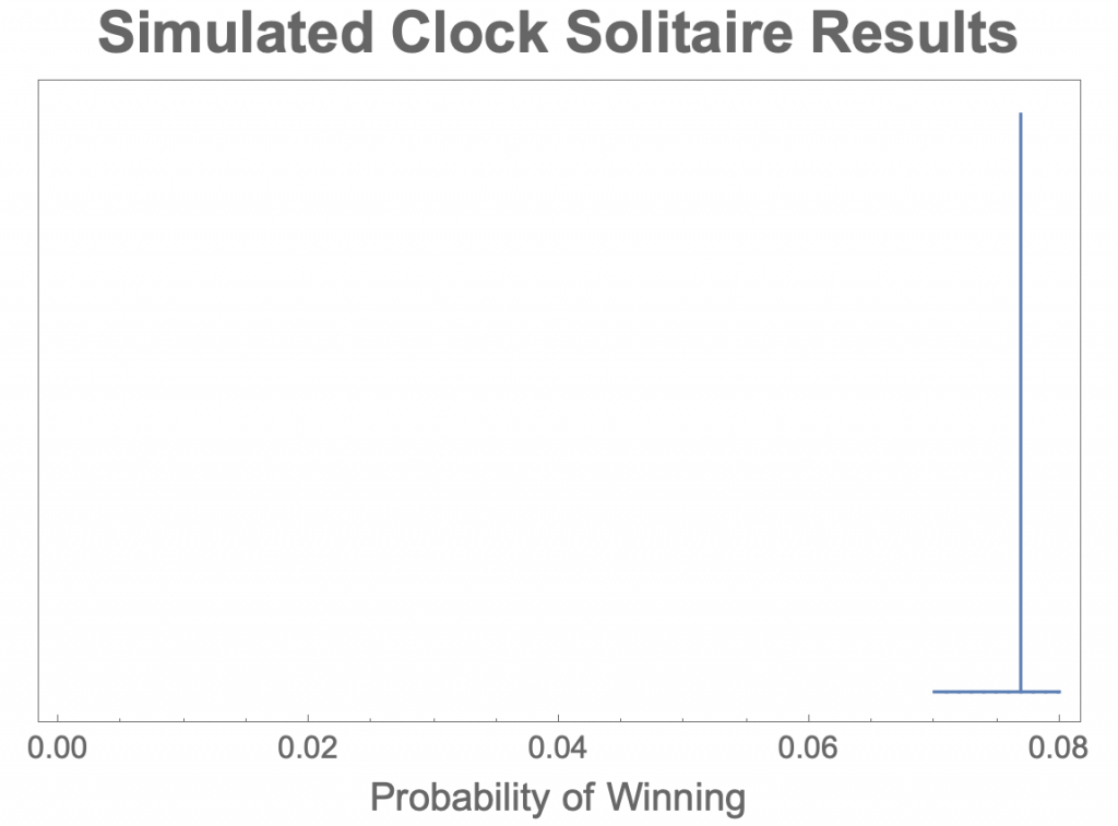
It turns out, that you the interval to contain 97% of the true probability values for my trillion simulations ranges from 0.076922 to 0.076924. In fact, my loyal steed Mathematica couldn’t even plot anything beyond what I showed you. So I had to switch to python (sigh). But that’s okay.
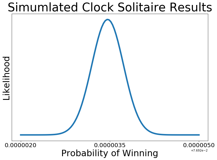
Anyways, the point is that I’m really, really certain (like 97% confident) that the actual probability of winning a game of clock solitaire falls between 7.6922% to 7.6924% from our work with a beta distribution. Again 1/13 = 0.076923….